A combo chart in Excel displays two chart types (such as column and line) on the same chart. They are used to show different types of information on a single chart, such as actuals against a target.

Excel中的组合图表在同一图表上显示两种图表类型(如柱形图和折线图)。 它们用于在单个图表上显示不同类型的信息，例如针对目标的实际值。

In this article, we’ll demonstrate how to make a combo chart that follows the same axis and one that displays mixed types of data in a single chart on a different axis.

在本文中，我们将演示如何制作一个沿同一轴的组合图表，以及一个在不同轴上的单个图表中显示混合数据类型的组合图表。

插入单轴组合图 (Insert a Combo Chart with a Single Axis)

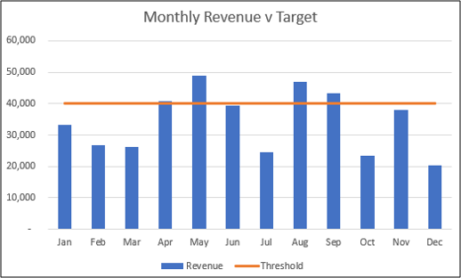
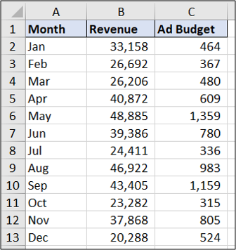
In the first example, we will create a combo chart to show monthly revenue against a target using the sample data below.

在第一个示例中，我们将使用下面的示例数据创建一个组合图，以显示针对目标的每月收入。

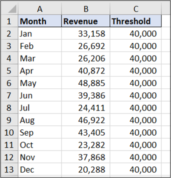
You can see that the target value is the same each month. The result will show the data as a straight line.

您可以看到每个月的目标值是相同的。 结果将数据显示为直线。

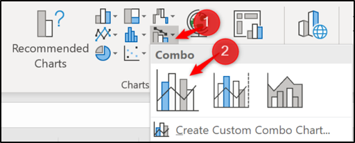
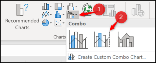
To get started, select the range of cells you want to chart—A1:C13 in this example. Next, click Insert > Insert Combo Chart. Select “Clustered Column – Line.”

首先，选择要绘制图表的单元格范围-在此示例中为A1：C13。 接下来，单击插入>插入组合图。 选择“群集列–行”。

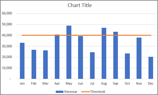
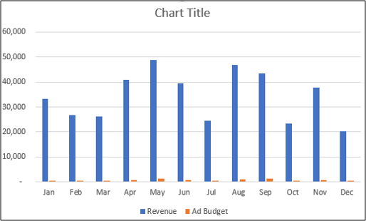
The combo chart is inserted with both the column and line using the same axis. Easy as that!

插入组合图时，列和线都使用相同的轴。 那样简单！

You can make further improvements to the chart now, like changing the chart title. Click on the chart title box and start typing to replace the words “Chart Title” with something more useful. As you type, the text will appear in the formula bar above.

您现在可以对图表进行进一步的改进，例如更改图表标题。 单击图表标题框，然后开始键入以将“ Chart Title”一词替换为更有用的名称。 键入时，文本将显示在上方的编辑栏中。

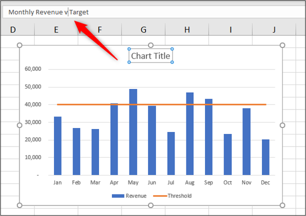
Press the Enter key, and Excel saves the typed text as the chart title.

按Enter键，然后Excel将键入的文本保存为图表标题。

插入带有两个轴的组合图 (Insert a Combo Chart with Two Axes)

Using the sample data shown below, let’s create a combo chart to show the monthly revenue and the ad budget on the same chart.

使用下面显示的示例数据，让我们创建一个组合图表，以在同一图表上显示每月收入和广告预算。

Select range A1:C13. Click Insert > Combo Chart. Choose the “Clustered Column – Line on Secondary Axis” chart.

选择范围A1：C13。 单击插入>组合图。 选择“聚集列–辅助轴上的线”图表。

The inserted chart looks like this.

插入的图表如下所示。

将现有图表更改为组合图表 (Change an Existing Chart to a Combo Chart)

We have looked at two examples of creating a combo chart from spreadsheet data, but knowing how to edit an existing chart can also be useful.

我们看了两个从电子表格数据创建组合图的示例，但是知道如何编辑现有图表也很有用。

Below is a clustered column chart created from the revenue and ad budget data.

以下是根据收入和广告预算数据创建的群集柱形图。

The chart has one axis, and you can barely see the ad budget columns on the chart. Let’s change this to a combo chart by creating a secondary axis for the ad budget data and changing its chart type to a line.

该图表有一个坐标轴，您几乎看不到图表上的广告预算列。 让我们通过为广告预算数据创建辅助轴并将其图表类型更改为折线，将其更改为组合图表。

To begin, right-click on the data series you want to change (ad budget in this example). Next, select “Change Series Chart Type.”

首先，右键单击要更改的数据系列(此示例中为广告预算)。 接下来，选择“更改系列图表类型”。

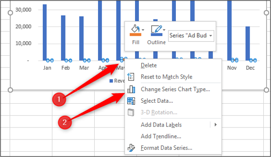
Now, check the “Secondary Axis” box for the data series you want to create an axis for. Select Line from the “Chart Type” list for that data series.

现在，在“辅助轴”框中选中要为其创建轴的数据系列。 从该数据系列的“图表类型”列表中选择“行”。

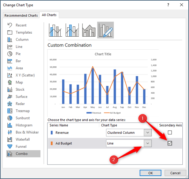
The chart is changed to a combo chart.

该图表将更改为组合图表。

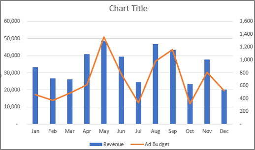
You can then make other improvements to the combo chart, such as editing the chart title or labeling the axis.

然后，您可以对组合图进行其他改进，例如编辑图表标题或标记轴。

翻译自: